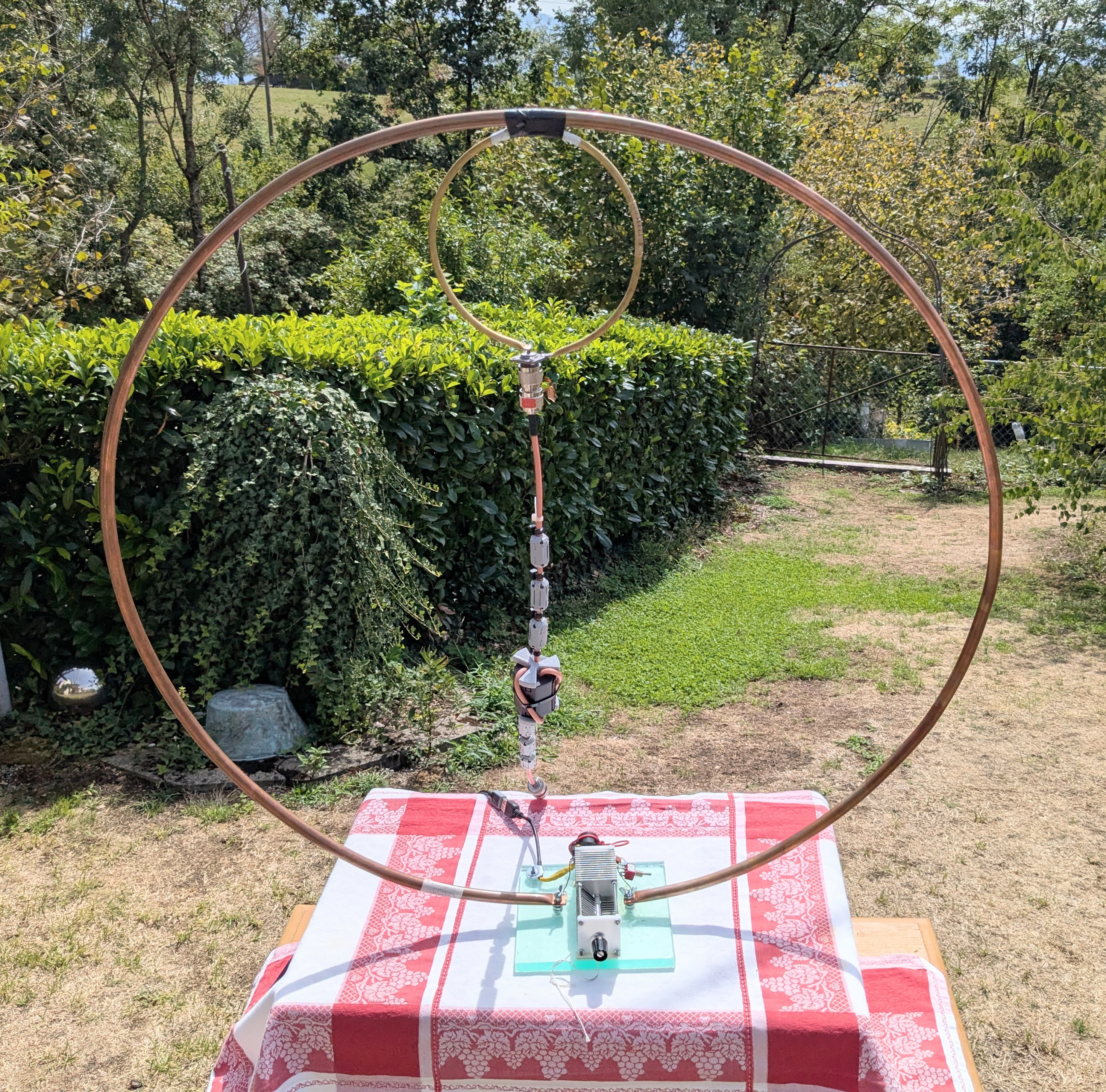
Info: Mag loop made of copper tubing with an air variable capacitor.
Conductor: Copper tube OD 12 mm, ID 10 mm, bare surface.
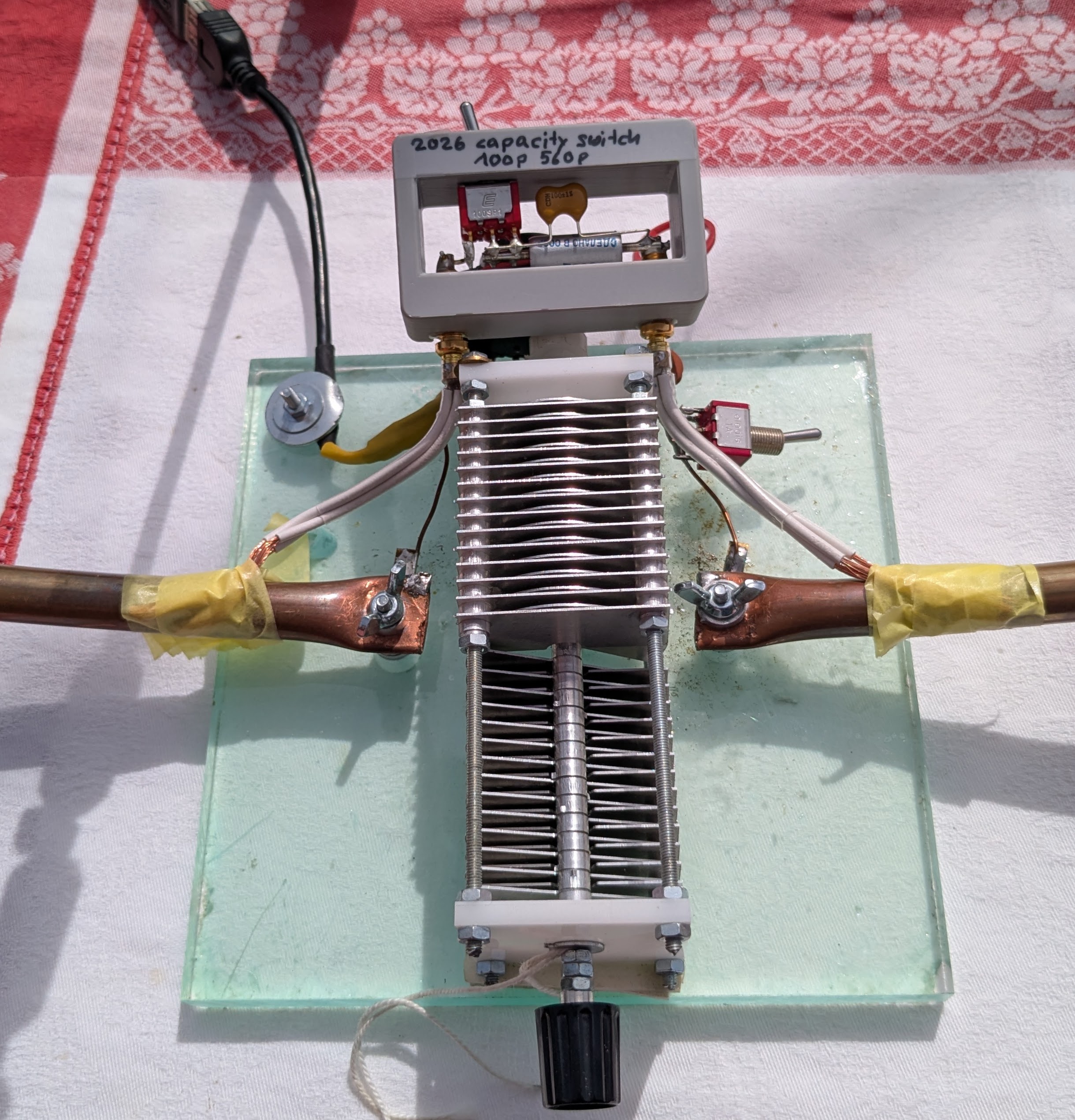
Capacitor: Air variable capacitor, self-made, CNC-milled from aluminum sheet.
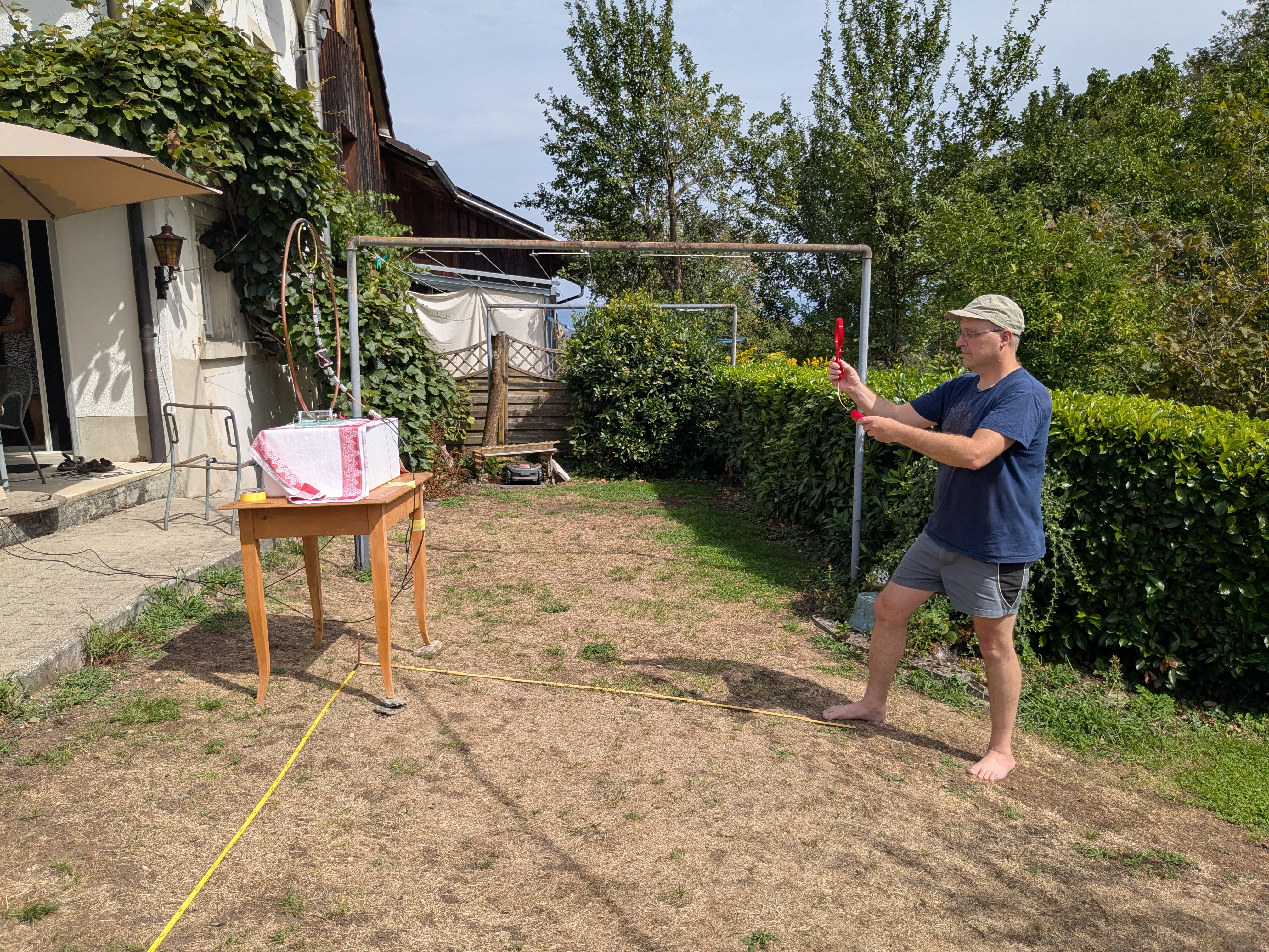
Environment: In the garden, on a Styrofoam box on a wooden table. Center loop 1.40 m above ground.
Thanks: Many thanks to Peter HB9BPO for the support, the fun conversations, and the catering.
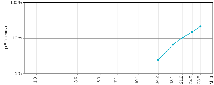
| Band | 20m | 17m | 15m | 12m | 10m | |
| Frequency f | MHz | 14.072 | 18.116 | 21.253 | 24.947 | 28.604 |
| Intrinsic bandwidth Bint | kHz | 99.1 | 102.7 | 123.6 | 165.6 | 201.9 |
| Source of Bint | S-Parameters | |||||
| Loop diameter D | m | 0.762 | ||||
| Conductor diameter d | m | 0.012 | ||||
| Loop count n | 1 | 1 | ||||
| Inductance L | H | 2.02e-06 | ||||
| Capacitance C | pF | 63.2 | 38.1 | 27.7 | 20.1 | 15.3 |
| Unloaded Q0 | 1 | 142 | 176 | 172 | 151 | 142 |
| Damping resistance RT | Ohm | 1.261 | 1.306 | 1.572 | 2.107 | 2.568 |
| Radiation resistance RR | Ohm | 0.0316 | 0.0872 | 0.166 | 0.316 | 0.550 |
| Loss resistance RLoss | Ohm | 1.229 | 1.219 | 1.406 | 1.790 | 2.018 |
| Power to antenna Pfwd | W | 10 | 10 | 10 | 10 | 10 |
| swr_min | 1 | 1.39 | 1.04 | 1.03 | 1.08 | 1.11 |
| etaSWR_ant | % | 97.4 | 100.0 | 100.0 | 99.9 | 99.7 |
| Power antenna load Pload | W | 10 | 10 | 10 | 10 | 10 |
| Antenna efficiency η | % | 2.44 | 6.67 | 10.5 | 15.0 | 21.4 |
| Loop current I rms | A | 2.78 | 2.77 | 2.52 | 2.18 | 1.97 |
| Loop voltage Uloop rms | V | 497 | 637 | 682 | 691 | 717 |
| Magnetic dipole moment m | A m² | 1.266 | 1.260 | 1.149 | 0.992 | 0.898 |
| Link to calculator | calculator | calculator | calculator | calculator | calculator | |
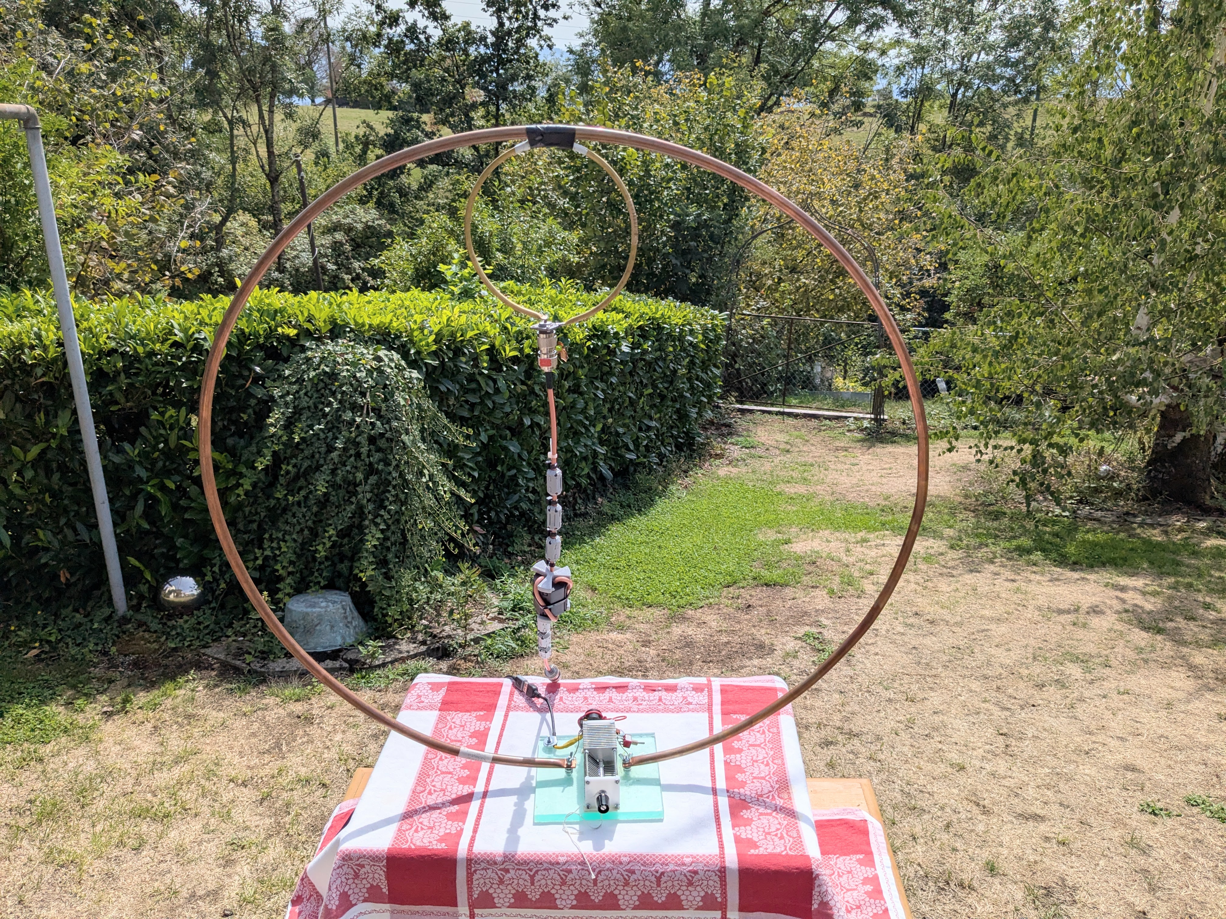
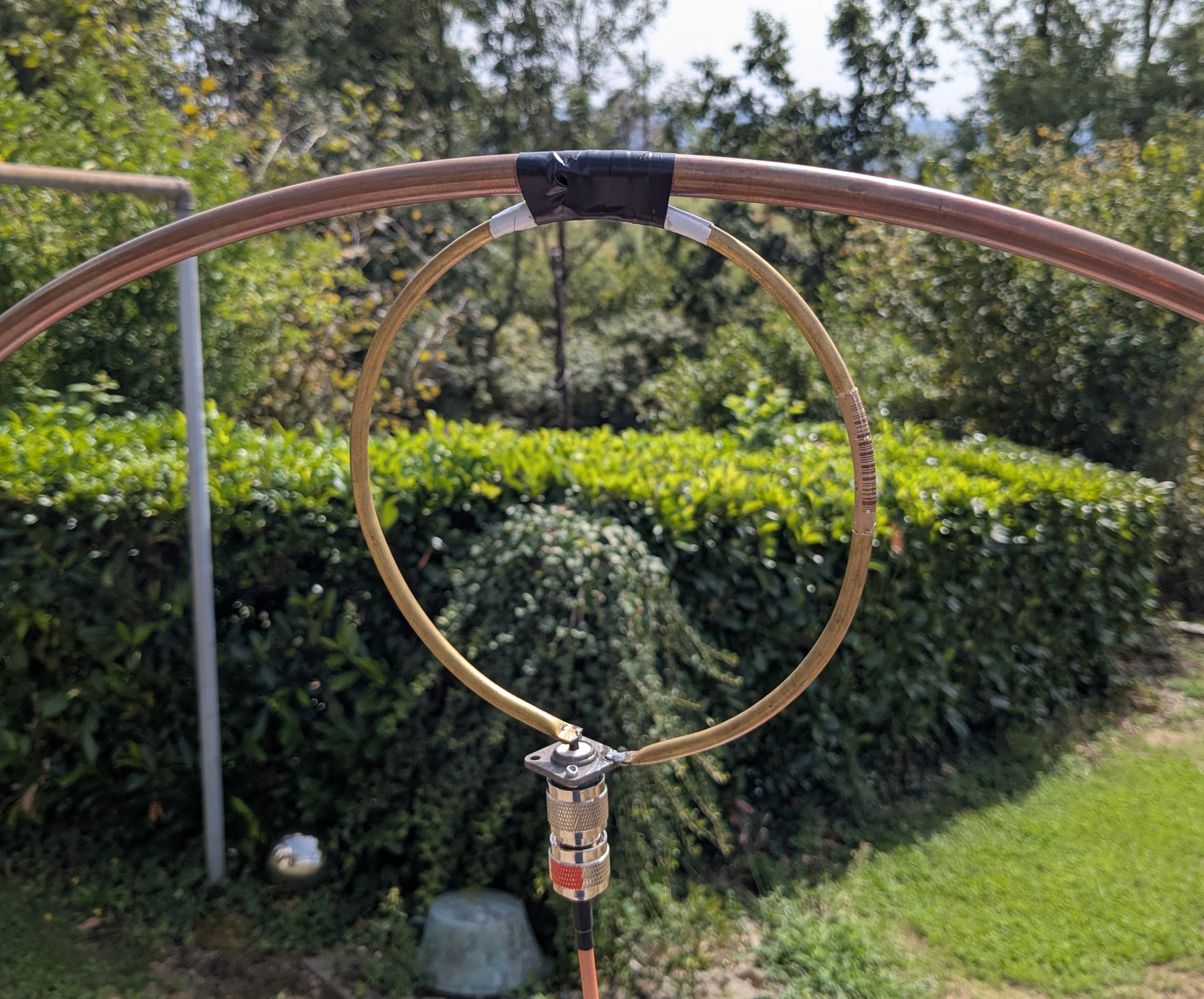
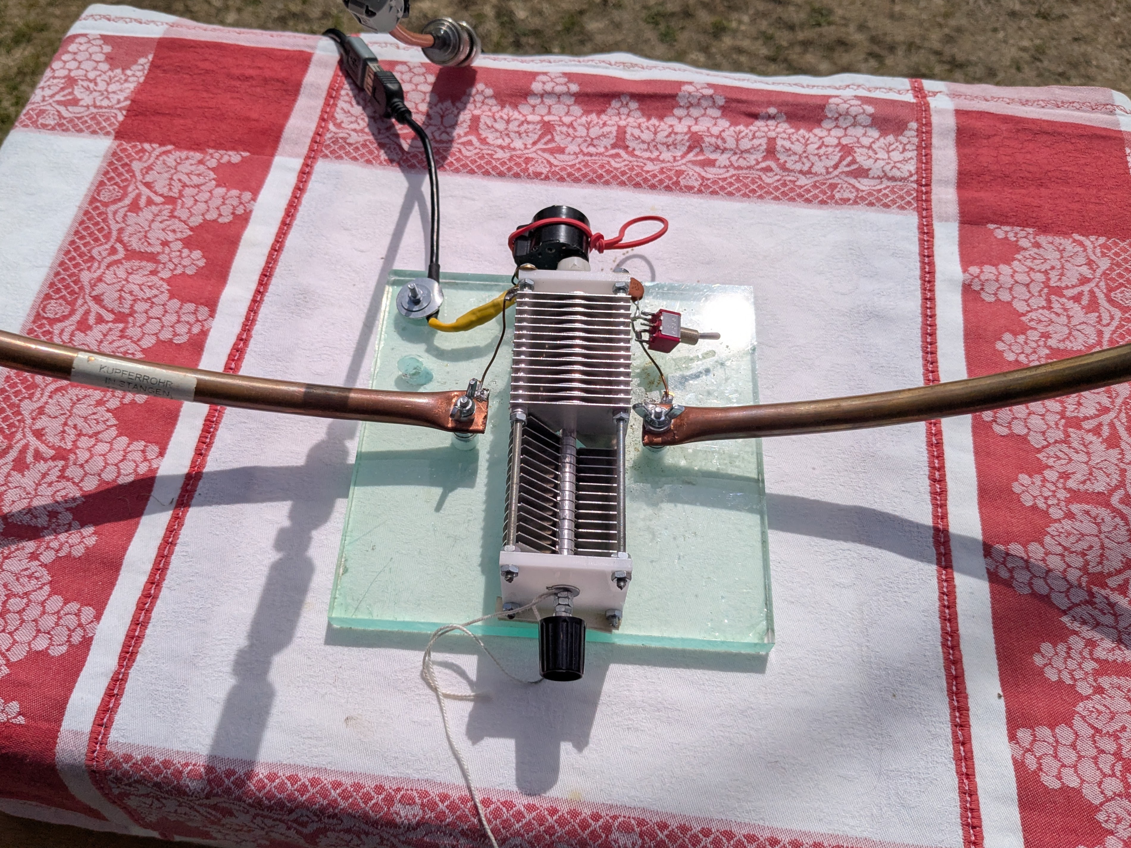
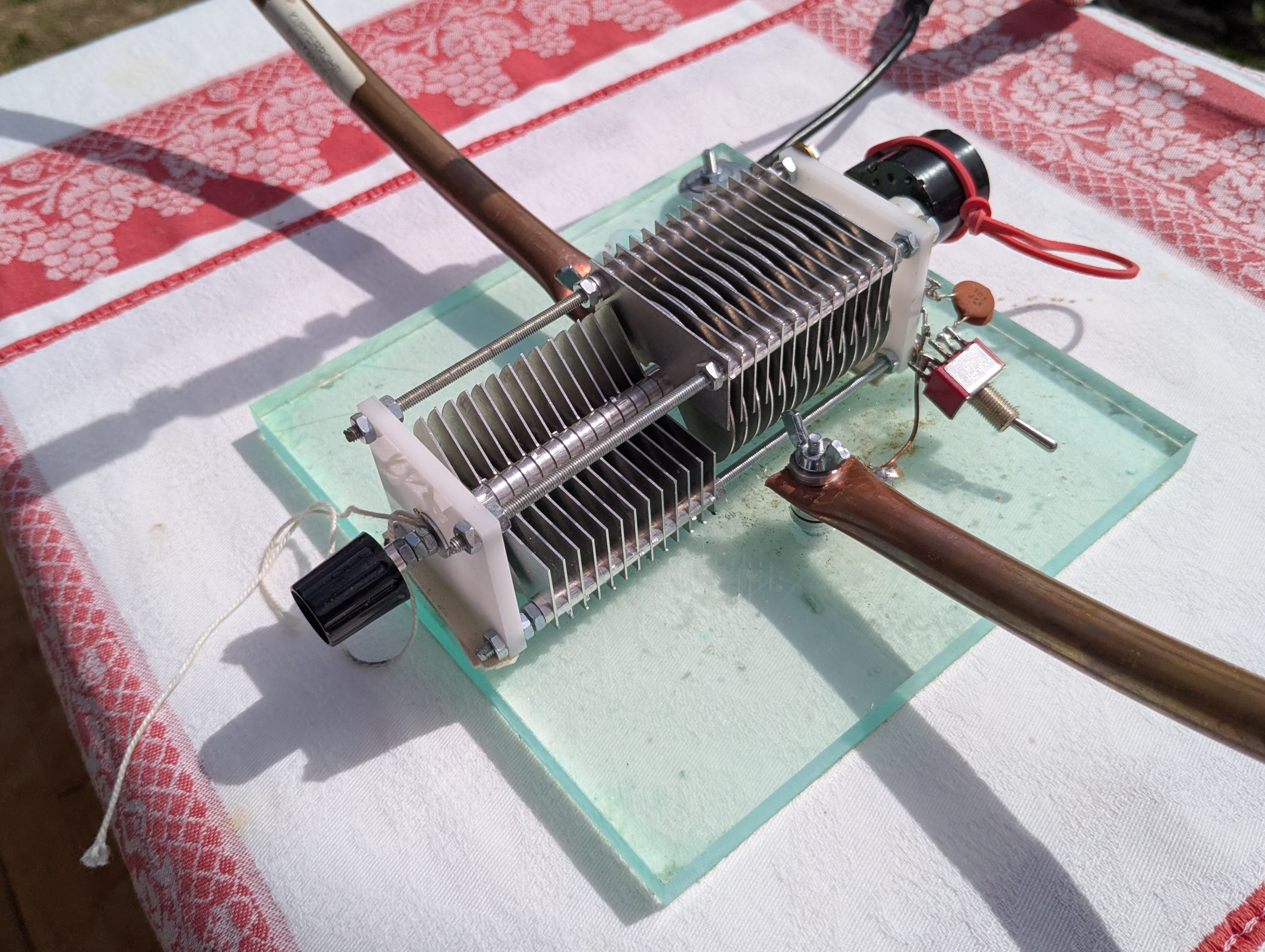
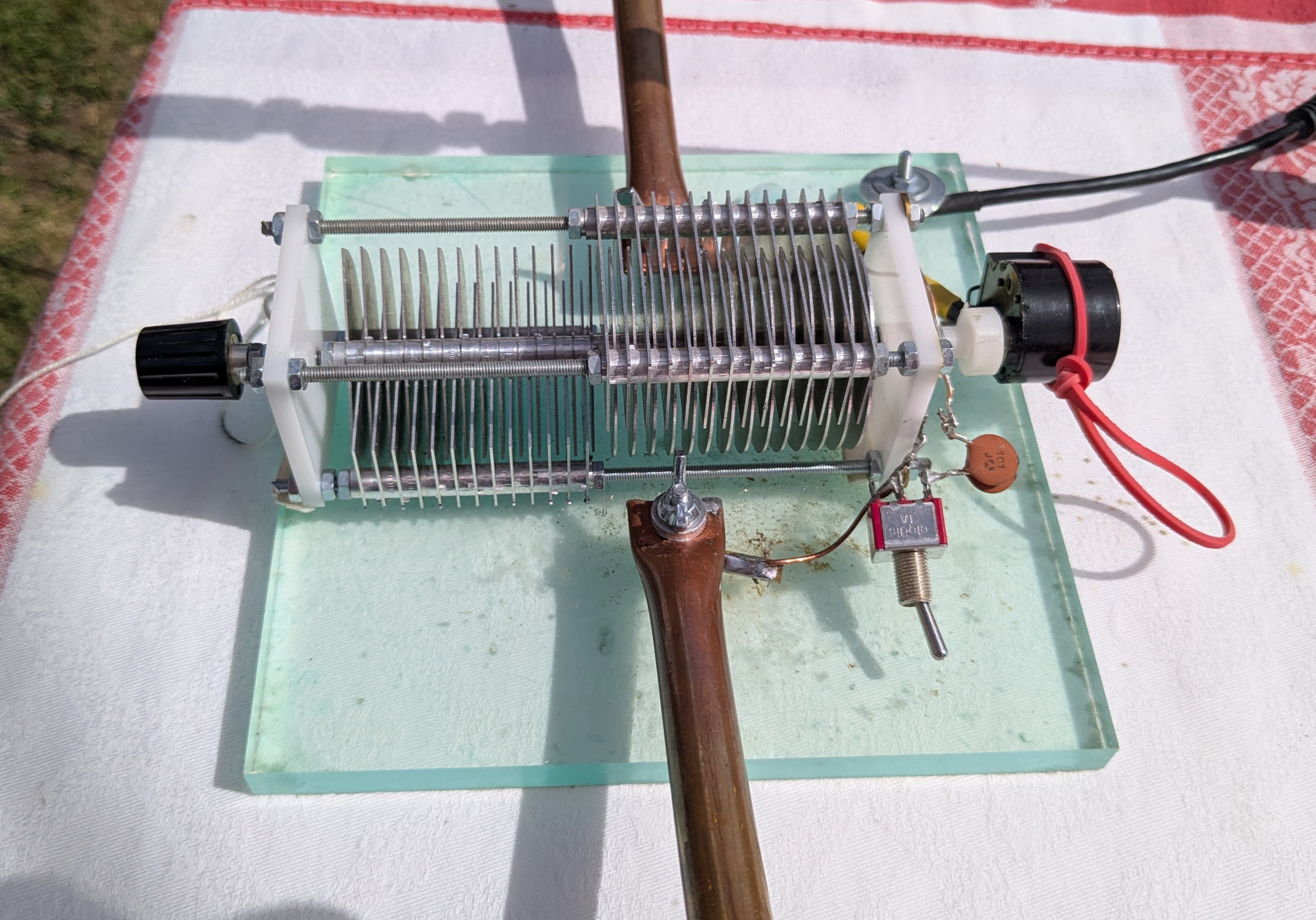
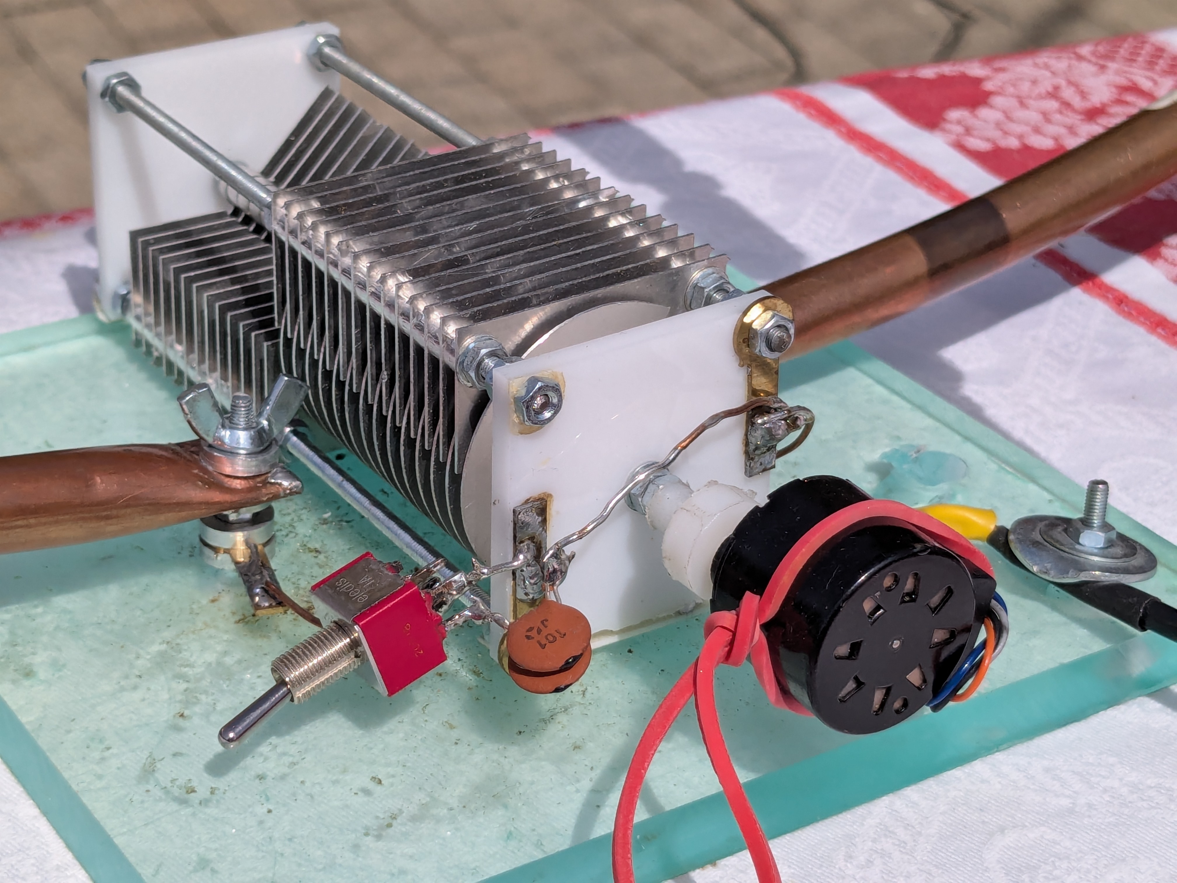
With the variable capacitor, the frequency can be tuned from 13.41 MHz up to 29.78 MHz.
The capacitor has external dimensions of approximately 40 mm x 40 mm x 220 mm.
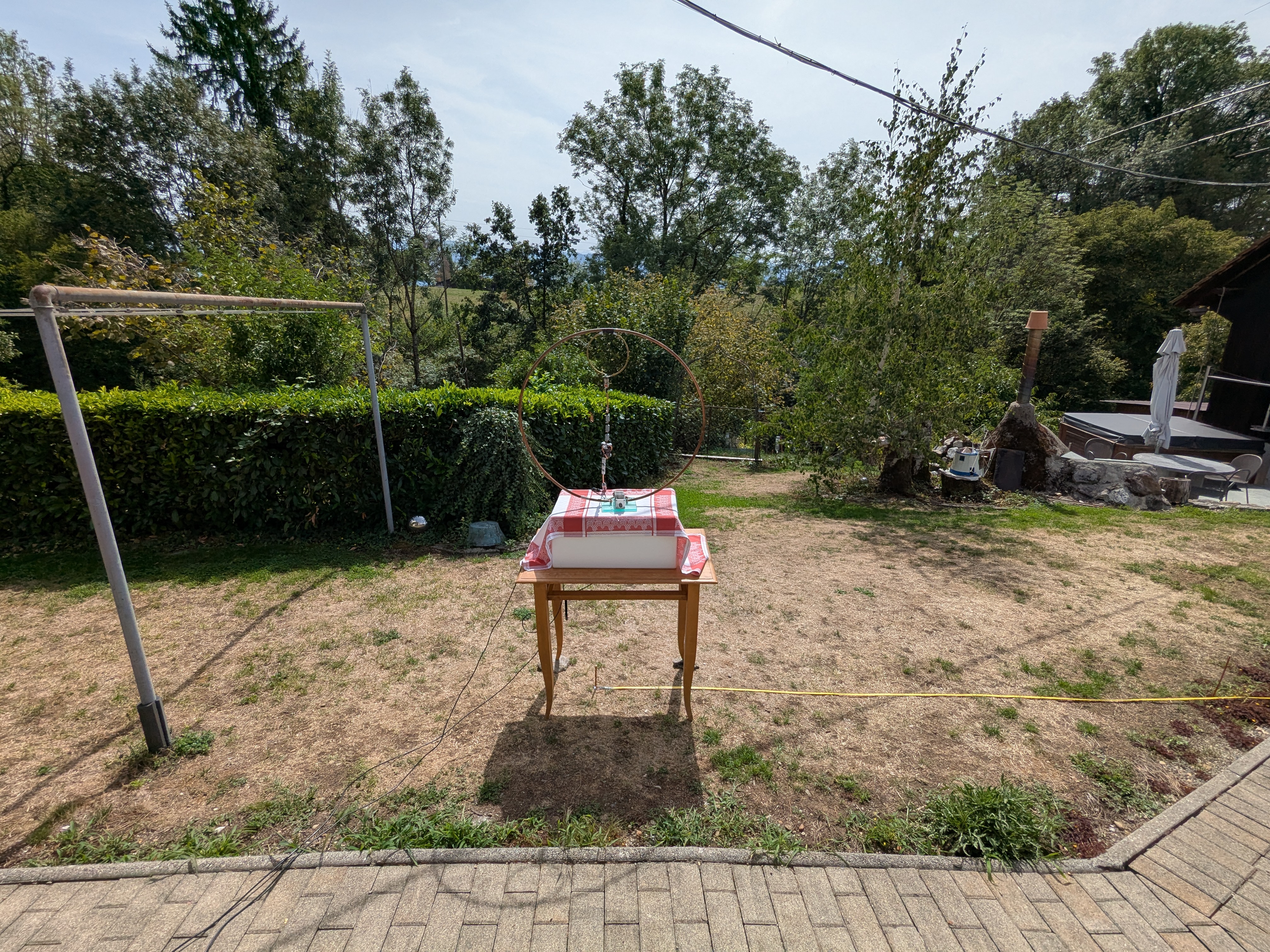
The loop center is 1.40 m above ground.
The nearest object in the surroundings is a clothesline post at a distance of about 2.5 m (visible on the left in the picture).
The grass is dry.
The antenna measurement setup is very practical. We sit at a table about 5 m away from the antenna.
A 10 m long LMR195 cable runs from the antenna to NanoVNA V2 Plus4.
Here we can also switch over to IC-7300 MK2 as transmitter.
For tuning, we measure the resonance with the VNA, and the capacitor is adjusted with a stepper motor.
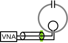
The calibration of the VNA was done at the antenna feed point: green line.
Common-mode choke at the antenna: positron.ch/rf/choke_simple
Used cables: 80 cm RG400 (including the choke) and 10 m LMR195.
The cable attenuation alpha and the cable delay tau in the following table should therefore be small.
| File | model f0 MHz |
model BSWR2_62 kHz |
model alpha db |
model_tau ns |
SWR min | eta SWR |
|---|---|---|---|---|---|---|
| 20260827_1344_antenne_14p1MHz_VALUES.py | 14.072 | 99.1 | 0.000 | 6.24 | 1.39 | 0.974 |
| 20260827_1409_antenne_28p6MHz_VALUES.py | 28.604 | 201.9 | 0.000 | 4.96 | 1.11 | 0.997 |
| 20260827_1419_antenne_24p9MHz_VALUES.py | 24.947 | 165.6 | 0.000 | 5.22 | 1.08 | 0.999 |
| 20260827_1426_antenne_21p3MHz_VALUES.py | 21.253 | 123.6 | 0.000 | 5.73 | 1.03 | 1.000 |
| 20260827_1435_antenne_18p1MHz_VALUES.py | 18.116 | 102.7 | 0.007 | 6.01 | 1.04 | 1.000 |
The following diagrams: red points = measured values; green line = fitted model.
| Smith | SWR | Values | ||||||||||||||||||
|---|---|---|---|---|---|---|---|---|---|---|---|---|---|---|---|---|---|---|---|---|
20260827_1344_antenne_14p1MHz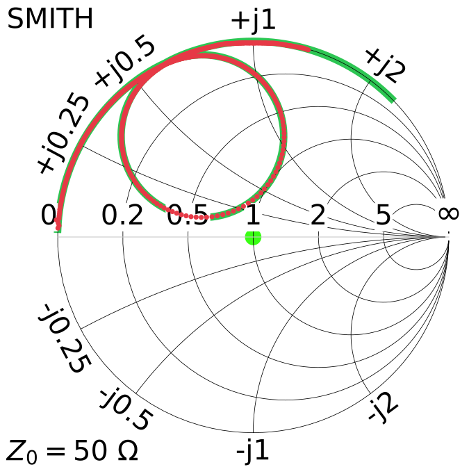 |
20260827_1344_antenne_14p1MHz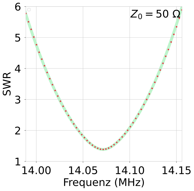 |
20260827_1344_antenne_14p1MHz
|
||||||||||||||||||
20260827_1409_antenne_28p6MHz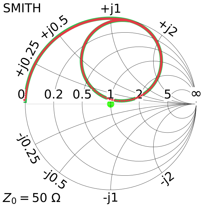 |
20260827_1409_antenne_28p6MHz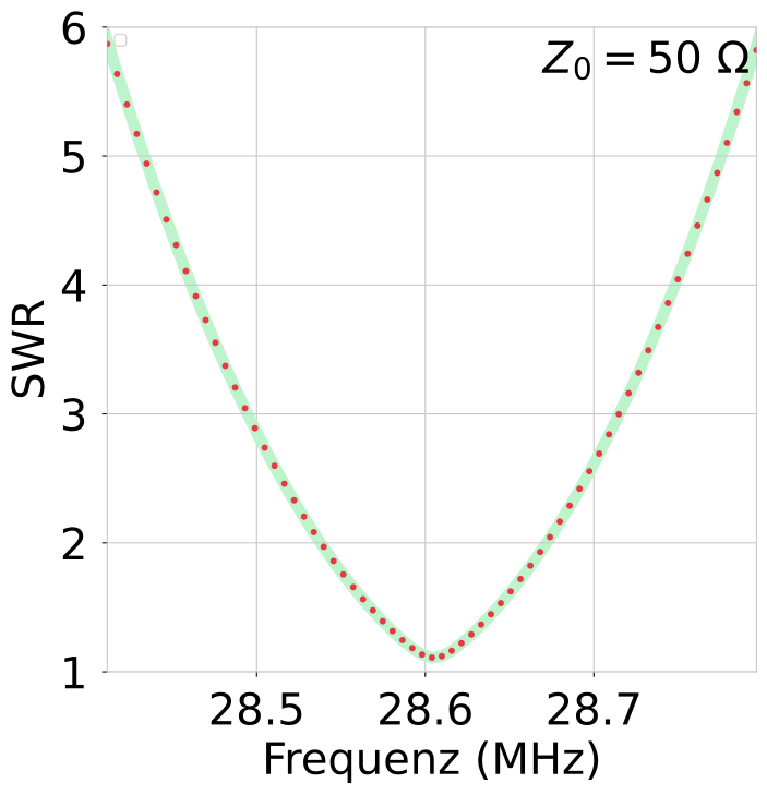 |
20260827_1409_antenne_28p6MHz
|
||||||||||||||||||
20260827_1419_antenne_24p9MHz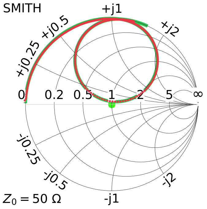 |
20260827_1419_antenne_24p9MHz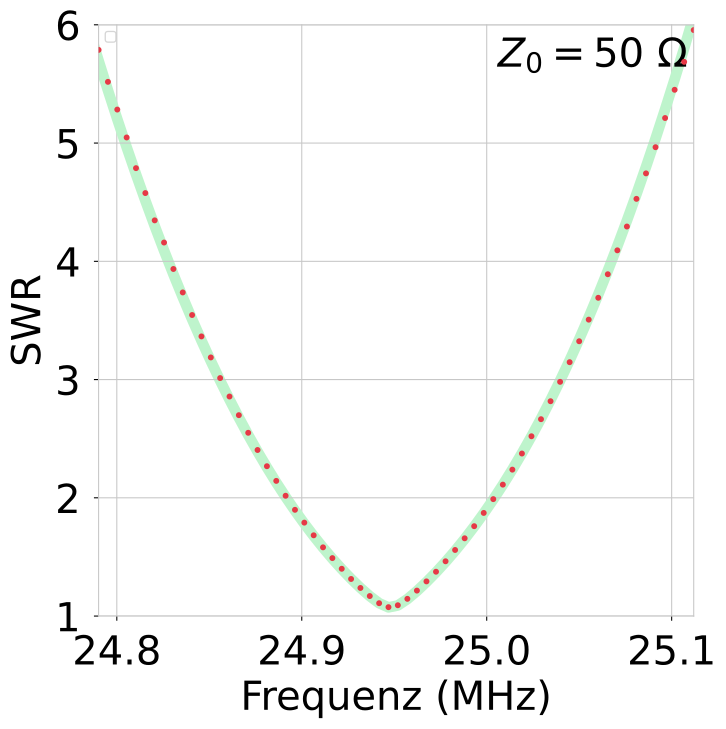 |
20260827_1419_antenne_24p9MHz
|
||||||||||||||||||
20260827_1426_antenne_21p3MHz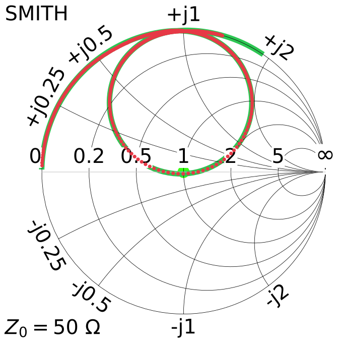 |
20260827_1426_antenne_21p3MHz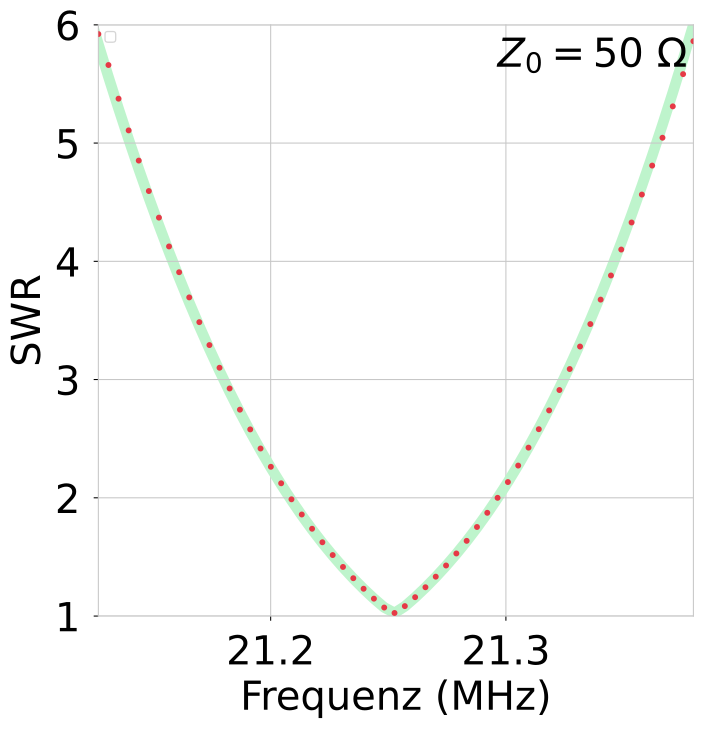 |
20260827_1426_antenne_21p3MHz
|
||||||||||||||||||
20260827_1435_antenne_18p1MHz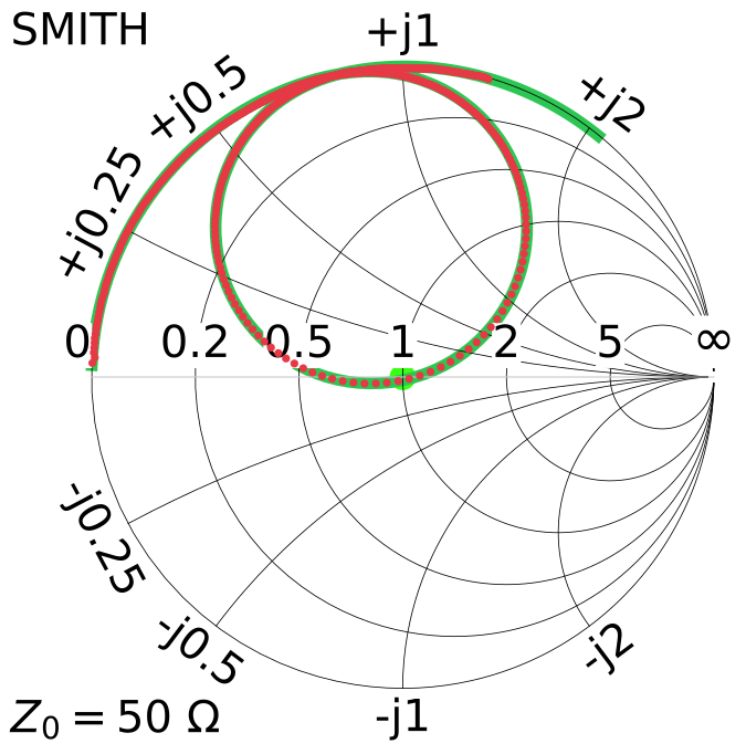 |
20260827_1435_antenne_18p1MHz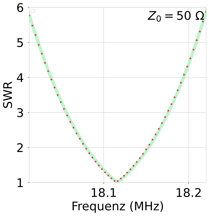 |
20260827_1435_antenne_18p1MHz
|
The main loop inductance is an important parameter because it directly affects the antenna efficiency calculation.
The inductance can be estimated from geometry (L). In general, an additional measurement is used as a cross-check, especially for non-circular loops where the geometric estimate is more difficult.
The resonance frequency of the LC circuit depends on L and C. Additional known capacitors are connected in parallel with the existing capacitor, and the new resonance frequency is measured.
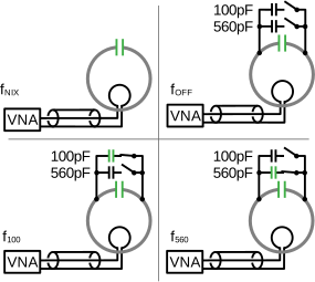
| fNIX | 18.112769 | MHz | Resonance frequency with no additional capacitors connected. |
| fOFF | 17.296894 | MHz | Capacitors and switches are physically connected at the antenna capacitor. A small parasitic capacitance from wiring and switches lowers the resonance frequency. |
| f100 | 9.369003 | MHz | Resonance frequency with an additional 100 pF capacitor switched in. |
| f560 | 4.450705 | MHz | Resonance frequency with an additional 560 pF capacitor switched in. |
| C100 | 100.0 | pF | Additional capacitance used for the 100 pF branch. |
| C560 | 579.0 | pF | Additional capacitance used for the 560 pF branch. |
| L | 2.024e-06 | H | Calculated from geometry of the main loop. |
| L100 | 2.039e-06 | H | Derived from the resonance frequencies fOFF and f100 deviation +1% vs L |
| L560 | 2.062e-06 | H | Derived from the resonance frequencies fOFF and f560 deviation +2% vs L |
| CNIX | 3.656e-12 | As/V | Derived from using L100, fOFF, and fNIX estimated parasitic capacitance of switches and wiring; expected value 1 ... 5 pF |
The maximum deviation between L and the capacitor-based L1x values is +2%. This is considered a small deviation and is accepted. L is used for the calculations of the antenna efficiency.
The H-field can be calculated under free-space conditions. In practice, however, the building contains numerous conductive objects that distort the field. To quantify the extent of this distortion, the H-field was measured and compared with the theoretical predictions.
The H-field is measured with a small measurement loop. The measuring setup is described in https://arxiv.org/abs/2607.10828.
A was used as the transmitter: 10 W, FM.
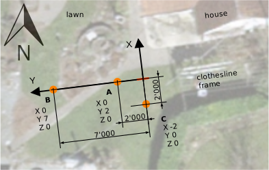
Even small deviations in position cause large changes in the measured value, because points A and C are very close to
the antenna and the field therefore changes rapidly.
At positions A and B, the field lines run exactly as expected from the theoretical free-space field-line pattern. At
position C, the field lines are tilted slightly upward (orientation of the measurement loop at maximum measured
value).
| tx_power_w | 10.0 |
| f_Hz | 14072000 |
| attenuation_cables_connectors_total_dbm | 0.76 dB |
| tx_after_cable_w | 8.4 |
| I_main_loop_A | 2.5 |
| magnetic dipole moment m (Am2) | 1.2 |
| X | Y | Z | expected | measured | factor | |
|---|---|---|---|---|---|---|
| m | m | m | A/m | A/m | ||
| A | 0.0 | 2.0 | 0.0 | 0.0113 | 0.0089 | 0.790 |
| B | 0.0 | 7.0 | 0.0 | 0.0010 | 0.0031 | 3.019 |
| C | -2.0 | 0.0 | 0.0 | 0.0237 | 0.0246 | 1.039 |
| tx_power_w | 10.0 |
| f_Hz | 18116000 |
| attenuation_cables_connectors_total_dbm | 0.83 dB |
| tx_after_cable_w | 8.3 |
| I_main_loop_A | 2.5 |
| magnetic dipole moment m (Am2) | 1.1 |
| X | Y | Z | expected | measured | factor | |
|---|---|---|---|---|---|---|
| m | m | m | A/m | A/m | ||
| A | 0.0 | 2.0 | 0.0 | 0.0104 | 0.0120 | 1.145 |
| B | 0.0 | 7.0 | 0.0 | 0.0018 | 0.0033 | 1.851 |
| C | -2.0 | 0.0 | 0.0 | 0.0267 | 0.0177 | 0.663 |
| tx_power_w | 10.0 |
| f_Hz | 21253000 |
| attenuation_cables_connectors_total_dbm | 0.89 dB |
| tx_after_cable_w | 8.2 |
| I_main_loop_A | 2.3 |
| magnetic dipole moment m (Am2) | 1.0 |
| X | Y | Z | expected | measured | factor | |
|---|---|---|---|---|---|---|
| m | m | m | A/m | A/m | ||
| A | 0.0 | 2.0 | 0.0 | 0.0095 | 0.0177 | 1.862 |
| B | 0.0 | 7.0 | 0.0 | 0.0022 | 0.0031 | 1.398 |
| C | -2.0 | 0.0 | 0.0 | 0.0271 | 0.0173 | 0.639 |
| tx_power_w | 10.0 |
| f_Hz | 24947000 |
| attenuation_cables_connectors_total_dbm | 0.95 dB |
| tx_after_cable_w | 8.0 |
| I_main_loop_A | 2.0 |
| magnetic dipole moment m (Am2) | 0.9 |
| X | Y | Z | expected | measured | factor | |
|---|---|---|---|---|---|---|
| m | m | m | A/m | A/m | ||
| A | 0.0 | 2.0 | 0.0 | 0.0093 | 0.0180 | 1.937 |
| B | 0.0 | 7.0 | 0.0 | 0.0027 | 0.0039 | 1.459 |
| C | -2.0 | 0.0 | 0.0 | 0.0256 | 0.0155 | 0.605 |
| tx_power_w | 10.0 |
| f_Hz | 28604000 |
| attenuation_cables_connectors_total_dbm | 1.00 dB |
| tx_after_cable_w | 7.9 |
| I_main_loop_A | 1.8 |
| magnetic dipole moment m (Am2) | 0.8 |
| X | Y | Z | expected | measured | factor | |
|---|---|---|---|---|---|---|
| m | m | m | A/m | A/m | ||
| A | 0.0 | 2.0 | 0.0 | 0.0102 | 0.0132 | 1.303 |
| B | 0.0 | 7.0 | 0.0 | 0.0032 | 0.0058 | 1.816 |
| C | -2.0 | 0.0 | 0.0 | 0.0249 | 0.0205 | 0.825 |
The measured field matches the free-space prediction reasonably well.
The largest deviations occur at point B.
This homebrew magnetic loop is a very nice DIY build.
It is lightweight, simple, and easy to transport.
The self-made capacitor with CNC-milled plates looks excellent and works flawlessly.
The coupling loop was already nearly perfectly matched from the start and was kept unchanged for all measurements.
The efficiency is not outstanding, but for the small loop diameter and simple construction it is appropriate.
There are probably many similar homebrew antennas around the world.
Overview of all Antennas with filter/selection: compare page
Overview of all Antennas static: static compare page
2026 Peter Märki (HB9ISP). This project is created in my free time and has no commercial background. Provided without warranty of any kind. Feedback is welcome.